

Mixture Model Trading (Part 5 - Algorithm Evaluation with pymc3)
/
Profitable Insights into Financial Markets
To see this weekend's prediction click here.
Overall this strategy has been impressive in its trial run over the last 4.5 weeks. I figured, given the volatility and uncertainty in the broad markets this week I'd like to see a mid-week update of the strategy using Python and the BarChart OnDemand API. To see my original article on the basics of using the BarChart OnDemand API click here.
First I import the basic modules needed to execute the script:
from copy import copy
import pandas as pd
import pandas_datareader.data as web
from pandas.tseries.offsets import *
From there I define a couple convenience functions. The first is a one off function for querying the BarChart API for singular symbol names. The other is a bulk function to aggregate the portfolio symbol price data into a HDF5 format for easy querying later on. Remember the api key is your api key.
# ================================================================== #
def _get_barChart_px(sym):
    start = '20160201'
    freq = 'minutes'
    api_url = construct_barChart_url(sym, start, freq, api_key=apikey)
    csvfile = pd.read_csv(api_url, parse_dates=['timestamp'])
    csvfile.set_index('timestamp', inplace=True)
    csvfile.index = csvfile.index.tz_localize('utc').tz_convert('US/Eastern')
    return csvfile
# ================================================================== #
def construct_barChart_url(sym, start_date, freq, api_key=apikey):
    '''Function to construct barchart api url'''
    url = 'http://marketdata.websol.barchart.com/getHistory.csv?' +\
            'key={}&symbol={}&type={}&startDate={}'.format(api_key, sym, freq, start_date)
    return url

# ================================================================== #
def get_minute_data(syms):
    '''Function to retrieve minute data for multiple stocks'''
    print('Running Get Minute Data')
    # This is the required format for datetimes to access the API
    # You could make a function to translate datetime to this format
    start = '20160201'
    #end = d
    freq = 'minutes'
    symbol_count = len(syms)
    N = copy(symbol_count)
    try:
        for i, sym in enumerate(syms, start=1):
            api_url = construct_barChart_url(sym, start, freq, api_key=apikey)
            try:
                csvfile = pd.read_csv(api_url, parse_dates=['timestamp'])
                csvfile.set_index('timestamp', inplace=True)
                # convert timestamps to EST
                csvfile.index = csvfile.index.tz_localize('utc').tz_convert('US/Eastern')
                symbol_store.put('{}'.format(sym), csvfile, format='table')
            except:
                continue
            N -= 1
            pct_total_left = (N/symbol_count)
            print('{}..[done] | {} of {} symbols collected | percent remaining: {:>.2%}'.format(sym, i, symbol_count, pct_total_left))
    except Exception as e:
        print(e)
    finally:
        pass
Next I run the function for aggregating the portfolio stocks prices.
longs = ['VO', 'GDX', 'XHB', 'XLB', 'HACK', 'XLY', 'XLP', 'XLU']
shorts = ['ACWI', 'VWO', 'IYJ', 'VB', 'VPU', 'ECH', 'VGK', 'IWB']

today = pd.datetime.today().date()
symbol_store = pd.HDFStore(price_path + 'Implied_Volatility_ETF_Tracking_{}.h5'.format(today.strftime('%m-%d-%y')))

symbols = longs+shorts
get_minute_data(symbols)
symbol_store.close()
After aggregating the data I perform some simple clean up operations along with calculation of the mid-prices for each minute of available data.
'''grab data from our previously created hdf5 file using keys'''
data = {}
loc = price_path + 'Implied_Volatility_ETF_Tracking_{}.h5'.format(today.strftime('%m-%d-%y'))
with pd.HDFStore(loc, 'r') as DATA:
    for key in DATA.keys():
        data[key] = DATA[key]
dat = pd.Panel.from_dict(data) # convert Python Dict to Pandas Panel

'''construct minute mid-prices'''
mids = pd.DataFrame()
for symbol in dat:
    mids[symbol] = (dat[symbol]['open'] + dat[symbol]['close']) / 2

'''Remove unnecessary forward slash from default HDF5 key label'''
cols = []
for sym in mids.columns:
    symz = sym.replace('/','')
    cols.append(symz)

mids.columns = cols
mids.head()
Because each ETF did not record a trade for every minute I perform a forward fill of the previous price before calculating the log returns. Then I calculate the cumulative sum of the the returns for both the long and short legs of the portfolio for comparison.
mids = mids.ffill()
lrets = np.log(mids / mids.shift(1))

crets = lrets.cumsum()
last_cret = crets.ix[-1]

long_rets = pd.Series()
for long in longs:
    long_rets.loc[long] = last_cret.loc[long]

short_rets = pd.Series()
for short in shorts:
    short_rets.loc[short] = last_cret.loc[short]
Finally, we arrive at the moment of truth. How has the strategy performed for the first 3 trading sessions of the week?
net_gain = long_rets.mean() - short_rets.mean()
print('long positions mean return: {:.3%}\nshort positions mean return: {:.3%}\ngross strategy pnl: {:.3%}'.format(long_rets.mean(), short_rets.mean(), net_gain))

Not bad at all! How does that compare to the US Major Market Averages? I perform almost the same process for the SPY, QQQ, and DIA ETF's except I use the singular BarChart API function defined above. I also calculate the mid-price for each minute of data.
'''get price data from BarChart'''
spy = _get_barChart_px('SPY')
qqq = _get_barChart_px('QQQ')
dia = _get_barChart_px('DIA')

'''calculate the midprice'''
spy_mid = (spy['open'] + spy['close']) / 2
qqq_mid = (qqq['open'] + qqq['close']) / 2
dia_mid = (dia['open'] + dia['close']) / 2

'''calculate the returns'''
spyr = np.log(spy_mid / spy_mid.shift(1))
qqqr = np.log(qqq_mid / qqq_mid.shift(1))
diar = np.log(dia_mid / dia_mid.shift(1))

'''calculate the cumulative sum of the returns'''
spyc = spyr.cumsum().ix[-1]
diac = diar.cumsum().ix[-1]
qqqc = qqqr.cumsum().ix[-1]

print('spy returns: {:.2%}\ndia returns: {:.2%}\nqqq returns: {:.2%}\nstrategy gross return: {:.2%}'.format(spyc, diac, qqqc, net_gain))
Wow! Not even close.

It's been a while since I've updated the blog and with good reason. Like any worthwhile business the foundation on which it's built must be thoroughly researched, well planned, and ruthlessly executed. With that in mind, I've been away building other pieces of the foundation which I will be unveiling over the next week or so. Be on the lookout for the upcoming BlackArbs flagship product titled the "iVC Report" (Identify Value Creators). This report is designed to assist retail and professional investors in their investment decisions by clearly identifying firms that create or destroy shareholder value.
The premise is simple; firms that create value always increase in value. Both sophisticated and unsophisticated investors are often confused about how to identify those stocks and as a result often make buy/sell decisions based on financial news media (awful), sell-side analysts (conflicts of interest), or their "gut" (erratic, emotion based). This report will help you cut through the profit destroying nonsense and provide the framework to improve the quality of your investment portfolio.
I will also be adding detailed valuation models as an add-on product in the next few weeks to further fortify the iVC report and BlackArbs' product offerings.
Also take note, I practice what I preach and use the iVC reports in all my investment decisions which has lead to risk adjusted outperformance compared to the S&P 500 over the last 2.5 quarters. As a result, I'm in the midst of constructing a core portfolio based entirely on my iVC reports and valuation process that I will update, track, and post so my current readers and prospective clients can follow along and see the results in real time.
I often consider the market's distortions that are or can be created by its participants. Arguably, the most important market player is the Federal Reserve. For years the FED as been injecting liquidity into the financial system through its Permanent Open Market Operations (POMO). I'm not going to delve into the purpose of these multibillion dollar transactions as others have covered this extensively. Instead I ask a simple question. The FED makes their tentative POMO schedule public beforehand. Can a trader simply buy the market open and sell the close each day the FED engages in POMO and earn a profit? The simple answer is 'yes'! To set up this study; I compared the FED"s historical POMO calender from January 2010 until August 3rd 2013 , to S&P 500 (SPX) returns for the matching dates. The return is based on a trader purchasing the SPX on open and closing the position at the end of day. I've provided the histogram of returns below along with an overlay of the density plot.
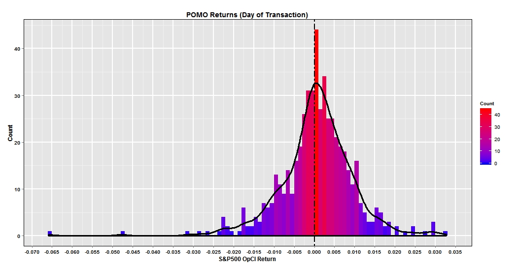
We can see that the returns have a slight negative skew with a couple >-4% days. Additionally the mode is just to the right of zero between 0 and 1%.. For context, the simple annualized sharp ratio is 0.51. Not great but slightly positive. I wondered if there could be a simple improvement to the strategy. What if the SPX trade was instead executed on the POMO settlement day which occurs the next trading day? The histogram below plots the return results.
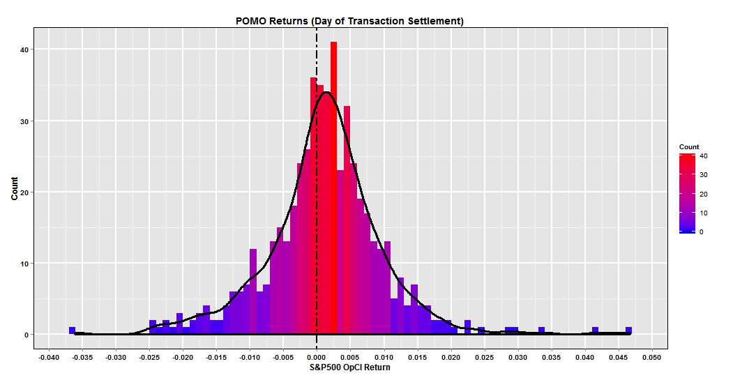
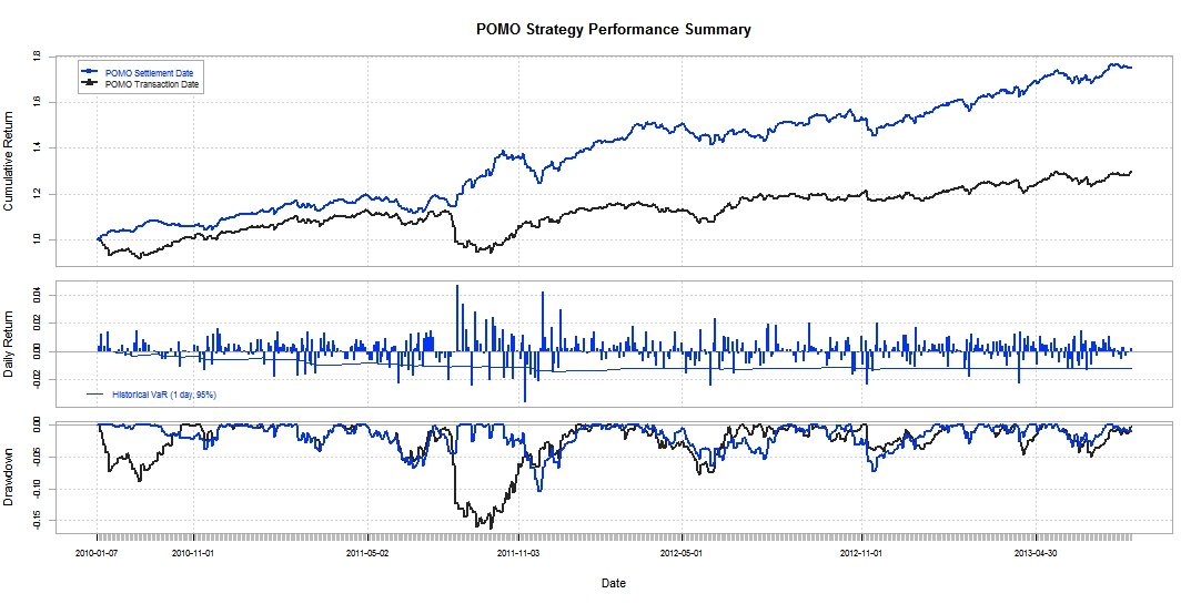
To my surprise this strategy was a large improvement. First there were no days with negative returns in excess of -4%. The mode is clearly positive approximating 2.5% and there appears to be a slight positive skew. For comparison the annualized Sharpe ratio is 1.76-Definitely respectable. Looking at the performance summary helps to compare the strategies. The first panel is a wealth index based on the cumulative value of $1 over the period. Clearly the settlement date strategy blows away the transaction date strategy by 40+% with a drawdown not exceeding 10% over the testing period.
Let me emphasize that the strategy may or may not be tradable today. On a superficial basis the strategy appears to be promising, But further research and more indepth analysis would have to be done, analyzing actual transactions, portfolio size, scale, and so on.
To construct the charts and run my analysis I used R!'s GGPLOT2 and PerformanceAnalytics packages along with Moments, Scales, and Quantmod.

AFFILIATE LINK
Powered by Squarespace