Does Factor Rank Matter for the Implied Volatility Skew Strategy?

Post Outline

• Strategy Summary
• Results
• Conclusions/Analysis

Strategy Summary

First, if you're unfamiliar with the Implied Volatility Skew Strategy you can find a recent deep dive into the strategy and its performance here.

In this short post, I look at the effect of using only the top N ranked ETFs from each Long/Short portfolio. In this case, N is equal to 3. This is an arbitrary selection and this study could be done with the top 1, 2, 4, etc. This differs from the original strategy in that the original strategy simply bins the ETFs into quantiles (according to the factor value) and creates the portfolio from the top and bottom quantiles; this strategy takes the top 3 ETFs from within the top and bottom quantiles.  

Results

I will reference the original strategy as S1 and the modified strategy as S2 for the remainder of the post.

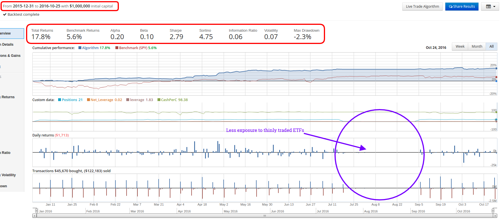
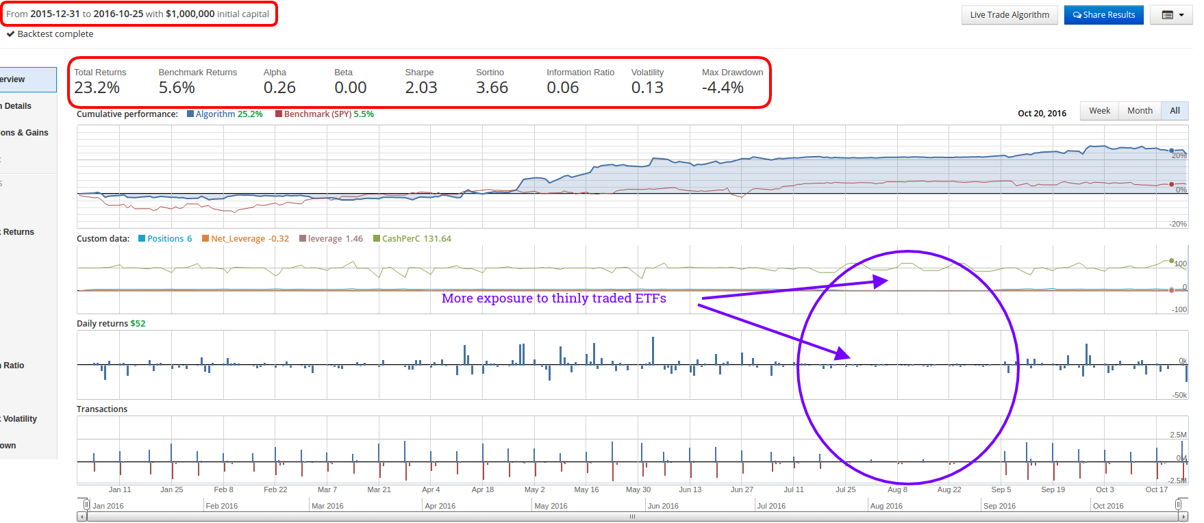
S1 is on the left and S2 is on the right.

View fullsize

View fullsize

S1 is on top and S2 is on the bottom.

Conclusions/Analysis

This strategy comparison exposes some key themes found in quant finance, but first some highlights:

• S2 outperforms S1 on a pure total return basis over the period. (~23% vs ~18%)
• S2 has a higher annualized alpha. (26% vs 20%)
• S2 has a lower annualized beta. (0% vs 10%)
• S2 has nearly double the volatility of S1. (13% vs 7%)
• S2 has nearly double the maximum drawdown of S1. (-4.4% vs -2.3%)
• S2 has max drawdown duration 3x larger than S1. (72 days vs 24 days)
• Both strategies have a positive information ratio of approximately 6%. 

We can extract a few lessons here.

S2 trades a maximum of six ETFs at a time vs the ~10+ ETFs of S1, so we would expect S2 to have a higher level of volatility than S1. You might ask, "Why is that?". Well, this is basic Market Portfolio Theory which relates diversification and portfolio volatility to the number of assets traded and their correlations with each other. Essentially, the theory says that the volatility of a portfolio of assets will be less than the sum of their individual volatility's as long as the correlations between the assets is not equal to 1. This is the power and benefit of diversification in a nutshell. 

Unfortunately for S2, the increase in total returns is not enough to compensate us for the increase in volatility (risk). This shows up primarily in the annualized sharpe ratio. S1 clearly has the edge in return per unit of risk, with a sharpe ratio of ~2.8 vs ~2. This also manifests in the Calmar ratio, which tracks the ratio of Avg. Annual Returns over Maximum Drawdown. Here S1 is also superior sporting a Calmar ratio of ~9.8 vs ~6.7.

S2's lower beta surprised me initially, but this is likely explained by trading less ETFs overall combined with those ETFs having low market correlation. 

Another issue we encounter with S2 vs S1 has to do with liquidity. In the equity curve charts, I have highlighted the general region where the strategy was on hiatus. Notice in S2, that there are tiny trades still occurring throughout this period. There should be no trades happening. What this means is that because S2 has to invest more cash into a smaller number of ETFs, if any of those ETFs are very thinly traded, it results in lots of unfilled orders that can take a significant amount of time to finish allocating or liquidating. Again, this is another side effect of S2's reduced diversification. 

Thus far all the evidence supports S1 as the superior strategy indicating that using a top N factor rank within top and bottom quantiles does not improve the strategy.