This post is a summary of a more detailed Jupyter (IPython) notebook where I demonstrate a method of using Python, Scikit-Learn and Gaussian Mixture Models to generate realistic looking return series. In this post we will compare real ETF returns versus synthetic realizations. To evaluate the similarity of the real and synthetic returns we will compare the following:

• visual inspection
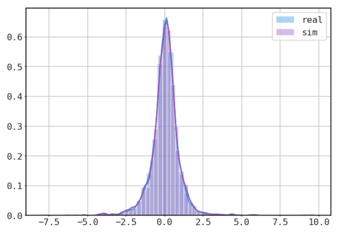
• histogram comparisons
• descriptive statistics
• correlations
• autocorrelations

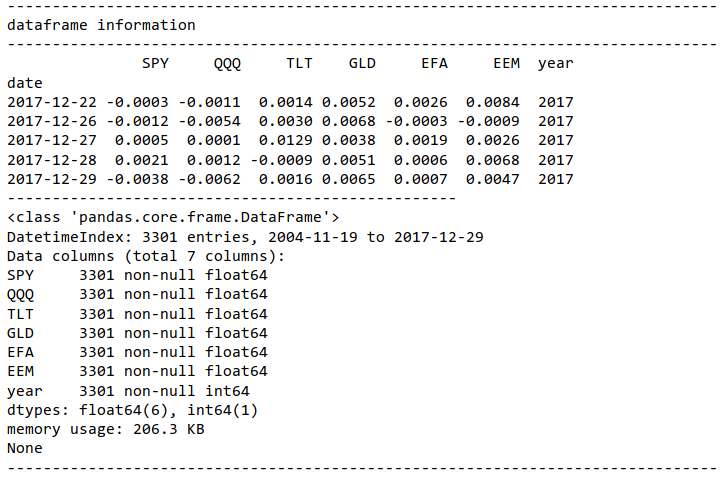
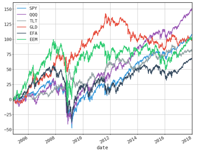
The data set we will use contains ETF daily data covering the period 2004 - 2017. The ETFs are SPY, QQQ, TLT, GLD, EFA, EEM, and the data is sourced from the Tiingo api.

Import Data

TIINGO DATA

Scale and Transform Data

Next we scale the data before fitting. I tried a few different methods including PCA (not technically a scaler), MaxAbsScaler, PowerTransformer, RobustScaler, and no scaling at all. Surprisingly the results were pretty similar with PowerTransformer and RobustScaler doing a slightly better job on the descriptive statistics. However my findings may be the result of randomness, thus I encourage the reader to experiment themselves.

Fit Mixture Model and Generate Simulation Path

Compare Real vs Synthetic

REAL

SYNTHETIC

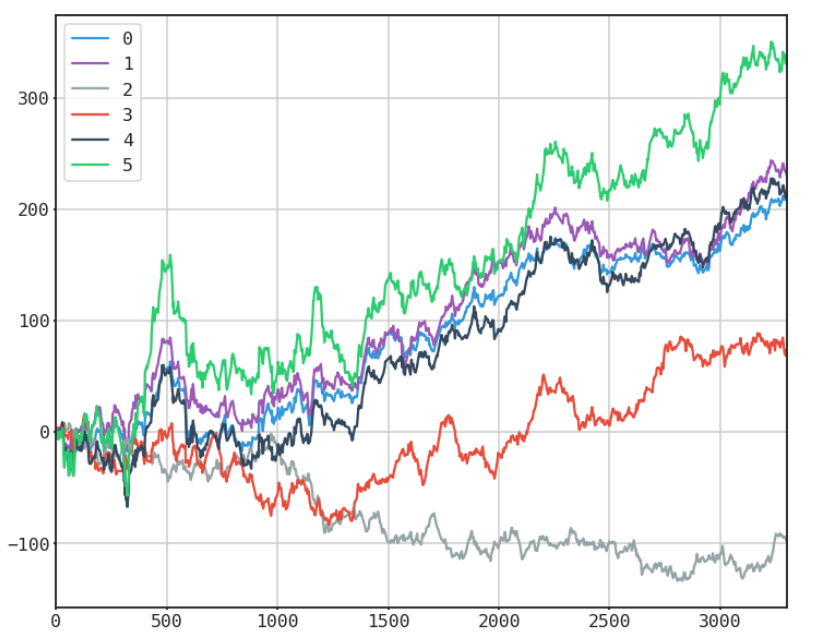
single random generation

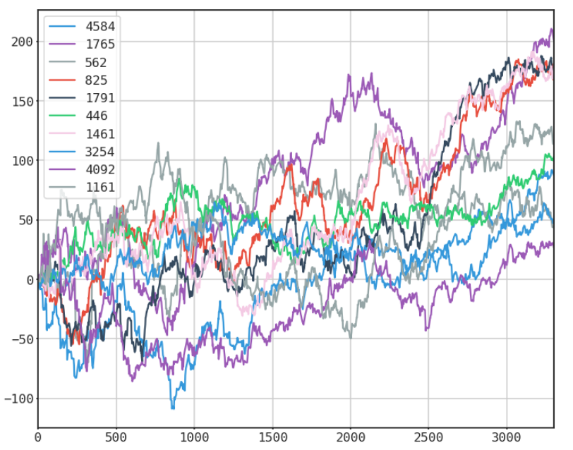
many selected random paths

COMPARE HISTOGRAMS

mean returns of single random generation vs mean returns of real returns

Not bad right? To see the detailed comparisons including the weaknesses of this approach view the notebook below or click the link to view it on nbviewer.org.

Jupyter Notebook Link

References

• In Depth: Gaussian Mixture Models by Jake VanderPlas