

Can We Use Mixture Models to Predict Market Bottoms? (Part 2)
/Post Outline
- Recap
- Model Update
- Model Testing
- Model Results
- Conclusions
- Code
Recap
In the previous post I gave a basic "proof" of concept, where we designed a trading strategy using Sklearn's implementation of Gaussian mixture models. The strategy attempts to predict an asset's return distribution such that returns that fall outside the predicted distribution are considered outliers and likely to mean revert. It showed some promise but had many areas in need of improvement.
Model Update
In this version I've refactored a lot of the code into a more object oriented structure. Now the code uses three classes.
- ModelRunner() class - This is the class for executing the model and returning our prediction dataframe and some key parameters.
- ResultEval() class - This takes the data from the prediction dataframe and key parameters and outputs our strategy returns and summary information.
- ModelPlots() class - This takes our data and outputs key plots to help visualize the strategy performance.
I did this for several reasons.
- Reduce the likelihood of input errors by creating objects that share parameters.
- Increase the ease of model testing.
- Increase interpretability.
Model Testing
In this version, we are going to expand the analysis to include other, actively traded ETFs, and test the reproducibility of the results, and generalization ability of the model.
Here are the ETFs we will examine:
symbols = ['SPY', 'DIA', 'QQQ', 'GLD', 'TLT', 'EEM', 'ACWI']
Assuming the correct imports, with the refactored code we can run the model in the following fashion. We'll focus on the TOO_LOW events although I encourage readers to experiment with both.
# Project Directory
DIR = 'YOUR/PROJECT/DIRECTORY/'

# get fed data
f1 = 'TEDRATE' # ted spread
f2 = 'T10Y2Y' # constant maturity ten yer - 2 year
f3 = 'T10Y3M' # constant maturity 10yr - 3m
factors = [f1, f2, f3]
ft_cols = factors + ['lret']

start = pd.to_datetime('2002-01-01')
end = pd.to_datetime('2017-01-01')

symbols = ['SPY', 'DIA', 'QQQ', 'GLD', 'TLT', 'EEM', 'ACWI']
for mkt in symbols:
    data = get_mkt_data(mkt, start, end, factors)

    # Model Params
    # ------------
    a, b = (.2, .7) # found via coarse parameter search
    alpha = 0.99
    max_iter = 100
    k = 2 # n_components
    init = 'random' # or 'kmeans'
    nSamples = 2_000
    year = 2009 # cutoff
    lookback = 1 # years
    step_fwd = 5 # days

    MR = ModelRunner(data, ft_cols, k, init, max_iter)
    dct = MR.prediction_cycle(year, alpha, a, b, nSamples)

    res = ResultEval(dct, step_fwd=step_fwd)
    event_dict = res._get_event_states()
    event = list(event_dict.keys())[1] # TOO_LOW

    post_events = res.get_post_events(event_dict[event])
    end_vals = res.get_end_vals(post_events)
    smry = res.create_summary(end_vals)

    p()
    p('*'*25)
    p(mkt, event.upper())
    p(smry.T)

    mp = ModelPlots(mkt, post_events, event, DIR, year)
    mp.plot_pred_results(dct['pred'], dct['year'], dct['a'], dct['b'])
    mp.plot_equity_timeline()
In this post I'm going to skip to the results and conclusions, and provide the refactored code at the end.
Model Results
First let's look at the model results using SPY.
The first thing I noticed was that the confidence intervals were less responsive to increases in return volatility. The difference shows up in the reduction in accuracy. In Part 1, I believe the accuracy was ~71% whereas in the updated model the accuracy has dipped to ~68%! Does that hurt our strategy?
Judging by the equity curve, our strategy is not noticeably impacted by the reduced model accuracy!
The plotted equity curve is the cumulative sum of each event's returns assuming every event was a "trade". This should include overlapping events.
Let's look at the model results for the other ETFs.
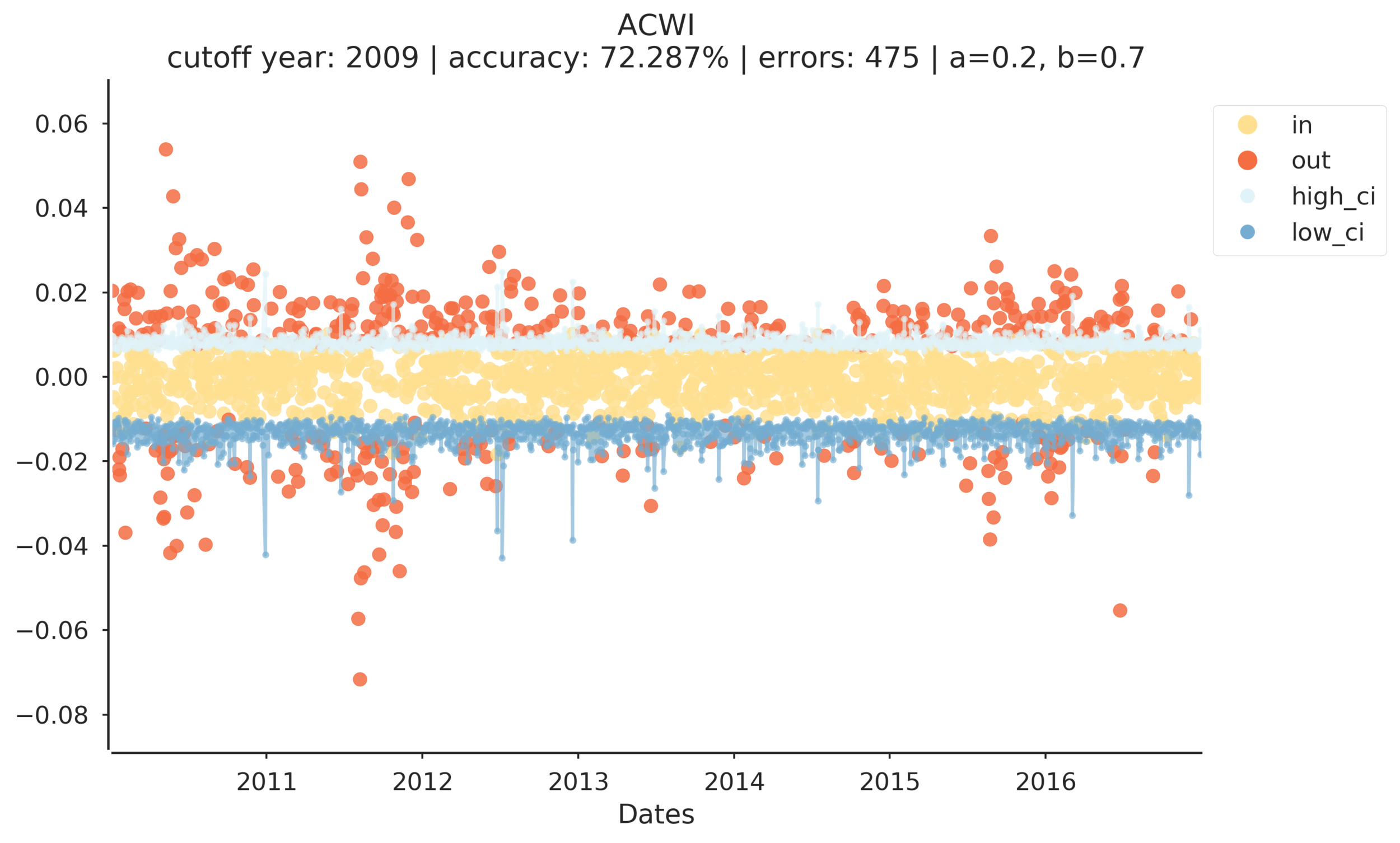


The model has some interesting output. Notice that model accuracy ranges from ~57% (TLT) to ~83% (EEM). However, both of these equity curves end positively. GLD is distinctly volatile, and ends poorly, however the model was 75% accurate. DIA, QQQ, SPY, and ACWI all have stable sharply positive equity curves.
Conclusions
This supports my initial findings that model accuracy seems loosely, if at all, related to the strategy's equity curve. These results do indicate that the strategy is worth further evaluation but I'm hesitant to declare success.
I need to test the strategy over a longer period of time and make sure to include 2008/9. Also, I need to drill down into evaluating the strategy results vs the correlation of asset returns. For example, DIA, QQQ, and SPY are highly correlated, so we would expect the strategy to have similar results among those ETFs, but what about negatively and uncorrelated assets? TLT is generally negatively correlated with SPY while GLD is likely uncorrelated. Is the strategy performance for those two ETFs representative of other negatively/uncorrelated ETFs?
Code
%load_ext watermark
%watermark
import pandas as pd
import pandas_datareader.data as web
import numpy as np
import sklearn.mixture as mix
import scipy.stats as scs

import matplotlib as mpl
import matplotlib.pyplot as plt
%matplotlib inline

import seaborn as sns
import missingno as msno
from tqdm import tqdm

import warnings
warnings.filterwarnings("ignore")
import affirm

sns.set(font_scale=1.25)
style_kwds = {'xtick.major.size': 3, 'ytick.major.size': 3,
              'font.family':u'courier prime code', 'legend.frameon': True}
sns.set_style('white', style_kwds)

p=print
p()
%watermark -p pandas,pandas_datareader,numpy,scipy,sklearn,matplotlib,seaborn
# **********************************************************************
def get_mkt_data(mkt, start, end, factors):
    """Function to get benchmark data from
        Yahoo and Factor data from FRED

    Params:
        mkt : str(), symbol
        start : pd.DateTime()
        end : pd.DateTime()
        factors : list() of str()
    Returns:
        data : pd.DataFrame()
    """
    MKT = (web.DataReader([mkt], 'yahoo', start, end)['Adj Close']
           .rename(columns={mkt:mkt})
           .assign(lret=lambda x: np.log(x[mkt]/x[mkt].shift(1)))
           .dropna())

    data = (web.DataReader(factors, 'fred', start, end)
            .join(MKT, how='inner')
            .dropna())
    return data
# **********************************************************************
class ModelRunner():
    def __init__(self, *args, **kwargs):
        """Class to run mixture model model

        Params:
            data : pd.DataFrame()
            ft_cols : list() of feature columns str()
            k : int(), n_components
            max_iter : int(), max iterations
            init : str() {random, kmeans}
        """
        self.data = data
        self.ft_cols = ft_cols
        self.k = k
        self.max_iter = max_iter
        self.init = init

        np.random.seed(123457)  # make results reproducible

    def _run_model(self, bgm=None, **kwargs):
        """Function to run mixture model

        Params:
            data : pd.DataFrame()
            ft_cols : list of str()
            k : int(), n_components
            max_iter : int()
            init : str() {random, kmeans}

        Returns:
            model : sklearn model object
            hidden_states : array-like, hidden states
        """
        X = self.data[self.ft_cols].values

        if bgm:
            model = mix.BayesianGaussianMixture(n_components=self.k,
                                                max_iter=self.max_iter,
                                                init_params=self.init,
                                                **kwargs,
                                               ).fit(X)
        else:
            model = mix.GaussianMixture(n_components=self.k,
                                        max_iter=self.max_iter,
                                        init_params=self.init,
                                        **kwargs,
                                       ).fit(X)

        hidden_states = model.predict(X)
        return model, hidden_states

    def _get_state_est(self, model, hidden_states):
        """Function to return estimated state mean and state variance

        Params:
            model : sklearn model object
            hidden_states : {array-like}
        Returns:
            mr_i : mean return of last estimated state
            mvar_i : model variance of last estimated state
        """
        # get last state
        last_state = hidden_states[-1]
        # last value is mean return for ith state
        mr_i = model.means_[last_state][-1]
        mvar_i = np.diag(model.covariances_[last_state])[-1]
        return mr_i, mvar_i

    def _get_ci(self, mr_i, mvar_i, alpha, a, b, nSamples):
        """Function to sample confidence intervals
            from the JohnsonSU distribution

        Params:
            mr_i : float()
            mvar_i : float()
            alpha : float()
            a : float()
            b : float()
            nsamples : int()
        Returns:
            ci : tuple(float(), float()), (low_ci, high_ci)
        """
        rvs_ = scs.johnsonsu.rvs(a, b, loc=mr_i, scale=mvar_i, size=nSamples)
        ci = scs.johnsonsu.interval(alpha=alpha, a=a, b=b,
                                    loc=np.mean(rvs_), scale=np.std(rvs_))
        return ci

    def prediction_cycle(self, *args, **kwargs):
        """Function to make walk forward predictions from cutoff year onwards

        Params:
            year : int(), cutoff year
            alpha : float()
            a : float()
            b : float()
            nsamples : int()
        Returns:
            dict() :
                pred : pd.DataFrame()
                year : str()
                a, b : float(), float()
        """
        cutoff = year
        train_df = self.data.ix[str(cutoff - lookback):str(cutoff)].dropna()
        oos = self.data.ix[str(cutoff+1):].dropna()
        # confirm that train_df end index is different than oos start index
        assert train_df.index[-1] != oos.index[0]

        # create pred list to hold tuple rows
        preds = []
        for t in tqdm(oos.index):
            if t == oos.index[0]:
                insample = train_df

            # run model func to return model object and hidden states using params
            model, hstates = self._run_model(**kwargs)
            # get hidden state mean and variance
            mr_i, mvar_i = self._get_state_est(model, hstates)
            # get confidence intervals from sampled distribution
            low_ci, high_ci = self._get_ci(mr_i, mvar_i, alpha, a, b, nSamples)
            # append tuple row to pred list
            preds.append((t, hstates[-1], mr_i, mvar_i, low_ci, high_ci))

            # increment insample dataframe
            insample = data.ix[:t]

        cols = ['ith_state', 'ith_ret', 'ith_var', 'low_ci', 'high_ci']
        pred = (pd.DataFrame(preds, columns=['Dates']+cols)
                .set_index('Dates').assign(tgt = oos['lret']))

        # logic to see if error exceeds neg or pos CI
        pred_copy = pred.copy().reset_index()
        # Identify indices where target return falls between CI
        win = pred_copy.query("low_ci < tgt < high_ci").index
        # create list of binary variables representing in/out CI
        in_rng_list = [1 if i in win else 0 for i in pred_copy.index]
        # assign binary variables sequence to new column
        pred['in_rng'] = in_rng_list
        return {'pred':pred, 'year':year, 'a':a, 'b':b}

# **********************************************************************
class ResultEval():
    def __init__(self, data, step_fwd):
        """Class to evaluate prediction results

        Params:
            data : dict() containing results of ModelRunner()
            step_fwd : int(), number of days to evalute post event
        """
        self.df = data['pred'].copy().reset_index()
        self.step_fwd=step_fwd

    def _get_event_states(self):
        """Function to get event indexes
        Index bjects must be called 'too_high', 'too_low'

        Returns:
            dict() : values are index objects
        """
        too_high = self.df.query("tgt > high_ci").index
        too_low = self.df.query("tgt < low_ci").index
        return {'too_high':too_high, 'too_low':too_low}

    def get_post_events(self, event):
        """Function to return dictionary where key, value is integer
        index, and Pandas series consisting of returns post event

        Params:
            df : pd.DataFrame(), prediction df
            event : {array-like}, index of target returns that exceed CI high or low
            step_fwd : int(), how many days to include after event
        Returns:
            after_event : dict() w/ values = pd.Series()
        """
        after_event = {}
        for i in range(len(event)):
            tmp_ret = self.df.ix[event[i]:event[i]+self.step_fwd, ['Dates','tgt']]
            # series of returns with date index
            after_event[i] = tmp_ret.set_index('Dates', drop=True).squeeze()
        return after_event

    def get_end_vals(self, post_events):
        """Function to sum and agg each post events' returns"""
        end_vals = []
        for k in post_events.keys():
            tmp = post_events[k].copy()
            tmp.iloc[0] = 0 # set initial return to zero
            end_vals.append(tmp.sum())
        return end_vals

    def create_summary(self, end_vals):
        """Function to take ending values and calculate summary
        Will fail if count of ending values (>0) or (<0) is less than 1
        """
        gt0 = [x for x in end_vals if x>0]
        lt0 = [x for x in end_vals if x<0]
        assert len(gt0) > 1
        assert len(lt0) > 1
        summary = (pd.DataFrame(index=['value'])
                   .assign(mean = f'{np.mean(end_vals):.4f}')
                   .assign(median = f'{np.median(end_vals):.4f}')
                   .assign(max_ = f'{np.max(end_vals):.4f}')
                   .assign(min_ = f'{np.min(end_vals):.4f}')
                   .assign(gt0_cnt = f'{len(gt0):d}')
                   .assign(lt0_cnt = f'{len(lt0):d}')
                   .assign(sum_gt0 = f'{sum(gt0):.4f}')
                   .assign(sum_lt0 = f'{sum(lt0):.4f}')
                   .assign(sum_ratio = f'{sum(gt0) / abs(sum(lt0)):.4f}')
                   .assign(gt_pct = f'{len(gt0) / (len(gt0) + len(lt0)):.4f}')
                   .assign(lt_pct = f'{len(lt0) / (len(gt0) + len(lt0)):.4f}')
                   )
        return summary
# **********************************************************************
class ModelPlots():
    def __init__(self, mkt, post_events, event_state, project_dir, year):
        """Class to visualize prediction results and summary

        Params:
            mkt : str(), symbol
            post_events : dict() of pd.Series()
            event_state : str(), 'too_high', 'too_low'
            project_dir : str()
            year : int(), cutoff year
        """
        self.mkt = mkt
        self.post_events = post_events
        self.event_state = event_state
        self.DIR = project_dir
        self.year = year

    def plot_equity_timeline(self):
        """Function to plot event timeline with equity curve second axis"""
        agg_tmp = []
        fig, ax = plt.subplots(figsize=(10, 7))
        ax1 = ax.twinx()
        ax.axhline(y=0, color='k', lw=3)
        for k in self.post_events.keys():
            tmp = self.post_events[k].copy()
            tmp.iloc[0] = 0 # set initial return to zero
            agg_tmp.append(tmp)
            if tmp.sum() > 0: color = 'dodgerblue'
            else: color = 'red'
            ax.plot(tmp.index, tmp.cumsum(), color=color, alpha=0.5)
            ax.set_xlim(pd.to_datetime(str(self.year) + '-12-31'), tmp.index[-1])
            ax.set_xlabel('Dates')
            ax.set_title(f"{self.mkt} {self.event_state.upper()}", fontsize=16)
            #sns.despine(offset=2)
        agg_df = pd.concat(agg_tmp).cumsum()
        ax1.plot(agg_df.index, agg_df.values, color='k', lw=5)
        ax.set_ylabel('Event Returns')
        ax1.set_ylabel('Equity Curve')
        fig.savefig(self.DIR + f'{self.mkt} {self.event_state.upper()} post events timeline {pd.datetime.today()}.png', dpi=300)
        return

    def plot_events_timeline(self):
        """Function to plot even timeline only"""
        fig, ax = plt.subplots(figsize=(10, 7))
        ax.axhline(y=0, color='k', lw=3)
        for k in self.post_events.keys():
            tmp = self.post_events[k].copy()
            tmp.iloc[0] = 0 # set initial return to zero

            if tmp.sum() > 0: color = 'dodgerblue'
            else: color = 'red'
            ax.plot(tmp.index, tmp.cumsum(), color=color, alpha=0.5)
            ax.set_xlim(pd.to_datetime('2009-12-31'), tmp.index[-1])
            ax.set_xlabel('Dates')
            ax.set_title(f"{self.mkt} {self.event_state.upper()}", fontsize=16, fontweight='demi')
            sns.despine(offset=2)
        fig.savefig(self.DIR + f'{self.mkt} {self.event_state.upper()} post events timeline.png', dpi=300)
        return

    def plot_events_post(self):
        """Function to plot events from zero until n days after"""
        fig, ax = plt.subplots(figsize=(10, 7))
        ax.axhline(y=0, color='k', lw=3)
        for k in self.post_events.keys():
            tmp = self.post_events[k].copy()
            tmp.iloc[0] = 0 # set initial return to zero

            if tmp.sum() > 0: color = 'dodgerblue'
            else: color = 'red'
            tmp.cumsum().reset_index(drop=True).plot(color=color, alpha=0.5, ax=ax)
        ax.set_xlabel('Days')
        ax.set_title(f"{self.mkt} {self.event_state.upper()}", fontsize=16, fontweight='demi')
        sns.despine(offset=2)
        fig.savefig(self.DIR + f'{self.mkt} {self.event_state.upper()} post events.png', dpi=300)
        return

    def plot_distplot(self, ending_values, summary):
        """Function to plot histogram of ending values"""
        colors = sns.color_palette('RdYlBu', 4)
        fig, ax = plt.subplots(figsize=(10, 7))
        sns.distplot(pd.DataFrame(ending_values), bins=15, color=colors[0],
                     kde_kws={"color":colors[3]}, hist_kws={"color":colors[3], "alpha":0.35}, ax=ax)
        ax.axvline(x=float(summary['mean'][0]), label='mean', color='dodgerblue', lw=3, ls='-.')
        ax.axvline(x=float(summary['median'][0]), label='median', color='red', lw=3, ls=':')
        ax.axvline(x=0, color='black', lw=1, ls='-')
        ax.legend(loc='best')
        sns.despine(offset=2)
        ax.set_title(f"{self.mkt} {self.event_state.upper()}", fontsize=16, fontweight='demi')
        fig.savefig(self.DIR + f'{self.mkt} {self.event_state.upper()} distplot.png', dpi=300)
        return

    def plot_pred_results(self, df, year, a, b):
        """Function to plot prediction results and confidence intervals"""
        # colorblind safe palette http://colorbrewer2.org/
        colors = sns.color_palette('RdYlBu', 4)

        fig, ax = plt.subplots(figsize=(10, 7))
        ax.scatter(df.index, df.tgt, c=[colors[1] if x==1 else colors[0] for x in df['in_rng']], alpha=0.85)
        df['high_ci'].plot(ax=ax, alpha=0.65, marker='.', color=colors[2])
        df['low_ci'].plot(ax=ax, alpha=0.65, marker='.', color=colors[3])
        ax.set_xlim(df.index[0], df.index[-1])

        nRight = df.query('in_rng==1').shape[0]
        accuracy = nRight / df.shape[0]
        ax.set_title('{:^10}\ncutoff year: {} | accuracy: {:2.3%} | errors: {} | a={}, b={}'
                      .format(self.mkt, year, accuracy, df.shape[0] - nRight, a, b))

        in_ = mpl.lines.Line2D(range(1), range(1), color="white", marker='o', markersize=10, markerfacecolor=colors[1])
        out_ = mpl.lines.Line2D(range(1), range(1), color="white", marker='o', markersize=10, markerfacecolor=colors[0])
        hi_ci = mpl.lines.Line2D(range(1), range(1), color="white", marker='.', markersize=15, markerfacecolor=colors[2])
        lo_ci = mpl.lines.Line2D(range(1), range(1), color="white", marker='.', markersize=15, markerfacecolor=colors[3])
        leg = ax.legend([in_, out_, hi_ci, lo_ci],["in", "out", 'high_ci', 'low_ci'],
                        loc = "center left", bbox_to_anchor = (1, 0.85), numpoints = 1)
        sns.despine(offset=2)
        file_str = self.DIR+f'{self.mkt} prediction success {pd.datetime.today()}.png'
        fig.savefig(file_str, dpi=300, bbox_inches="tight")
        return
