

Can We Use Mixture Models to Predict Market Bottoms? (Part 3)
/Post Outline
- Recap
- Webinar Hypothesis
- Anaylsis/Conclusions
- Jupyter (IPython) Notebook
- Github Links and Resources
Recap
Thus far in the series we've explored the idea of using Gaussian mixture models (GMM) to predict outlier returns. Specifically, we were measuring two things:
- The accuracy of the strategy implementation in predicting return distributions.
- The return pattern after an outlier event.
During the exploratory phase of this project there were some interesting results worthy of more investigation. The initial results implied that the strategy implementation was adaptable to changes in the means and volatilities of a small number of ETF's returns.
Webinar Hypothesis
Recently I had the opportunity to present my first webinar with QuantInsti.com. I definitely have some areas for improvement, but the experience was great overall, and I learned a lot.
I chose this topic to present, and through the process I was able to refine the hypothesis, the code, and my thinking on the subject. The hypothesis is simple:
Can a GMM based strategy predict asset return distributions such that a strategy which "buys" the asset post an outlier event can "earn" a positive return?
Analysis and Conclusions
There were a couple of takeaways from the project. Overall the strategy showed promise. What really impressed me was the difference in the sampled confidence intervals when using the Normal distribution vs. the JohnsonSU distribution. See the following example:


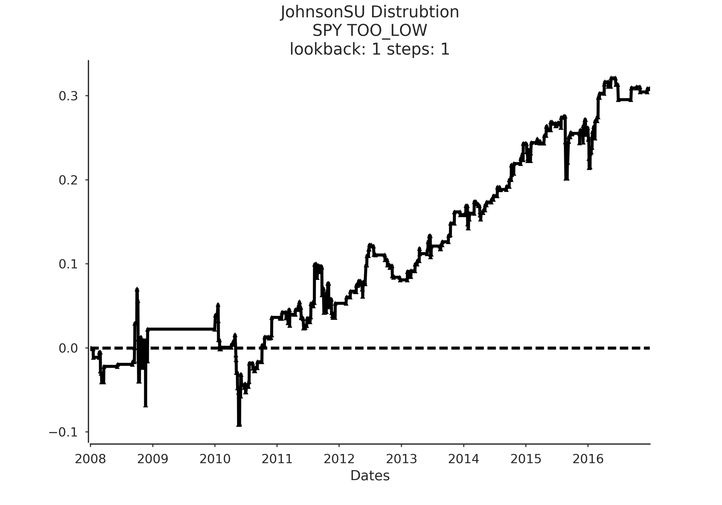
On the left, we have the same strategy except the sampled confidence intervals are drawn from a normal distribution. On the right we use the JohnsonSU distribution. In terms of predicted return distribution accuracy it's not even close-JohnsonSU is the clear winner, even showing an ability to adjust to periods of clustered volatility.
However note the equity curves in the example. The normal distribution wins handily but that is because the strategy is so inaccurate that it predicts outlier returns occurred ~97% of the time, so technically that would be a buy and hold strategy which benefits from the strong uptrend in SPY post 2009.
Another takeaway is that the model shows a bias towards US based ETFs. You can see that by examining the Seaborn facetgrid plots in the notebook I will share at the end. First, by aggregating the results in to a tidy-data format the analysis was rendered so simple, I kicked myself for not adhering to these principles sooner. In the examples I examine the strategy results according to median returns and the sum_ratio.
Median returns are simply the median returns of the strategy for that set of parameters. The sum_ratio is the sum of all strategy returns that ended positively divided by the sum of all returns that ended negatively for a set of parameters. A "successful" strategy should have a sum_ratio > 1 across multiple dimensions as well as consistent positive median returns.
In the analysis I look at the two metrics across different lookback periods (1 year, 3 year, and expanding), different numbers of mixture model components (k=2, 3, 5, 7, 9, 13, 17, 21) and across a number of holding periods in days (steps = 1, 2, 3, 5, 7, 10, 21).
When applied to SPY, QQQ, and TLT the strategy showed consistent positive results across a wide spectrum of parameter combinations whereas the application to GLD, EFA, and EEM were a little more mixed and definitely not as encouraging.
One theory I have for this result is that the factors I used as input to the GMM are US based interest rate spreads. These are likely to have a much stronger relationship to the behavior of SPY, QQQ, TLT vs the other ETFs. To improve performance I believe one would have to locate indicators based on the asset/ETF one wants to trade.
To sum up, I'm encouraged by the strategy framework, but would like to see a wider array of stocks, asset classes, and ETFs tested with various combinations of factors.
Jupyter (IPython) Notebook
Here is a sample exploratory notebook I put together for the webinar that demonstrates the conclusions drawn above.
