

Exploring Alternative Price Bars
/
Profitable Insights into Financial Markets
To see this weekend's prediction click here.
Overall this strategy has been impressive in its trial run over the last 4.5 weeks. I figured, given the volatility and uncertainty in the broad markets this week I'd like to see a mid-week update of the strategy using Python and the BarChart OnDemand API. To see my original article on the basics of using the BarChart OnDemand API click here.
First I import the basic modules needed to execute the script:
from copy import copy
import pandas as pd
import pandas_datareader.data as web
from pandas.tseries.offsets import *
From there I define a couple convenience functions. The first is a one off function for querying the BarChart API for singular symbol names. The other is a bulk function to aggregate the portfolio symbol price data into a HDF5 format for easy querying later on. Remember the api key is your api key.
# ================================================================== #
def _get_barChart_px(sym):
    start = '20160201'
    freq = 'minutes'
    api_url = construct_barChart_url(sym, start, freq, api_key=apikey)
    csvfile = pd.read_csv(api_url, parse_dates=['timestamp'])
    csvfile.set_index('timestamp', inplace=True)
    csvfile.index = csvfile.index.tz_localize('utc').tz_convert('US/Eastern')
    return csvfile
# ================================================================== #
def construct_barChart_url(sym, start_date, freq, api_key=apikey):
    '''Function to construct barchart api url'''
    url = 'http://marketdata.websol.barchart.com/getHistory.csv?' +\
            'key={}&symbol={}&type={}&startDate={}'.format(api_key, sym, freq, start_date)
    return url

# ================================================================== #
def get_minute_data(syms):
    '''Function to retrieve minute data for multiple stocks'''
    print('Running Get Minute Data')
    # This is the required format for datetimes to access the API
    # You could make a function to translate datetime to this format
    start = '20160201'
    #end = d
    freq = 'minutes'
    symbol_count = len(syms)
    N = copy(symbol_count)
    try:
        for i, sym in enumerate(syms, start=1):
            api_url = construct_barChart_url(sym, start, freq, api_key=apikey)
            try:
                csvfile = pd.read_csv(api_url, parse_dates=['timestamp'])
                csvfile.set_index('timestamp', inplace=True)
                # convert timestamps to EST
                csvfile.index = csvfile.index.tz_localize('utc').tz_convert('US/Eastern')
                symbol_store.put('{}'.format(sym), csvfile, format='table')
            except:
                continue
            N -= 1
            pct_total_left = (N/symbol_count)
            print('{}..[done] | {} of {} symbols collected | percent remaining: {:>.2%}'.format(sym, i, symbol_count, pct_total_left))
    except Exception as e:
        print(e)
    finally:
        pass
Next I run the function for aggregating the portfolio stocks prices.
longs = ['VO', 'GDX', 'XHB', 'XLB', 'HACK', 'XLY', 'XLP', 'XLU']
shorts = ['ACWI', 'VWO', 'IYJ', 'VB', 'VPU', 'ECH', 'VGK', 'IWB']

today = pd.datetime.today().date()
symbol_store = pd.HDFStore(price_path + 'Implied_Volatility_ETF_Tracking_{}.h5'.format(today.strftime('%m-%d-%y')))

symbols = longs+shorts
get_minute_data(symbols)
symbol_store.close()
After aggregating the data I perform some simple clean up operations along with calculation of the mid-prices for each minute of available data.
'''grab data from our previously created hdf5 file using keys'''
data = {}
loc = price_path + 'Implied_Volatility_ETF_Tracking_{}.h5'.format(today.strftime('%m-%d-%y'))
with pd.HDFStore(loc, 'r') as DATA:
    for key in DATA.keys():
        data[key] = DATA[key]
dat = pd.Panel.from_dict(data) # convert Python Dict to Pandas Panel

'''construct minute mid-prices'''
mids = pd.DataFrame()
for symbol in dat:
    mids[symbol] = (dat[symbol]['open'] + dat[symbol]['close']) / 2

'''Remove unnecessary forward slash from default HDF5 key label'''
cols = []
for sym in mids.columns:
    symz = sym.replace('/','')
    cols.append(symz)

mids.columns = cols
mids.head()
Because each ETF did not record a trade for every minute I perform a forward fill of the previous price before calculating the log returns. Then I calculate the cumulative sum of the the returns for both the long and short legs of the portfolio for comparison.
mids = mids.ffill()
lrets = np.log(mids / mids.shift(1))

crets = lrets.cumsum()
last_cret = crets.ix[-1]

long_rets = pd.Series()
for long in longs:
    long_rets.loc[long] = last_cret.loc[long]

short_rets = pd.Series()
for short in shorts:
    short_rets.loc[short] = last_cret.loc[short]
Finally, we arrive at the moment of truth. How has the strategy performed for the first 3 trading sessions of the week?
net_gain = long_rets.mean() - short_rets.mean()
print('long positions mean return: {:.3%}\nshort positions mean return: {:.3%}\ngross strategy pnl: {:.3%}'.format(long_rets.mean(), short_rets.mean(), net_gain))

Not bad at all! How does that compare to the US Major Market Averages? I perform almost the same process for the SPY, QQQ, and DIA ETF's except I use the singular BarChart API function defined above. I also calculate the mid-price for each minute of data.
'''get price data from BarChart'''
spy = _get_barChart_px('SPY')
qqq = _get_barChart_px('QQQ')
dia = _get_barChart_px('DIA')

'''calculate the midprice'''
spy_mid = (spy['open'] + spy['close']) / 2
qqq_mid = (qqq['open'] + qqq['close']) / 2
dia_mid = (dia['open'] + dia['close']) / 2

'''calculate the returns'''
spyr = np.log(spy_mid / spy_mid.shift(1))
qqqr = np.log(qqq_mid / qqq_mid.shift(1))
diar = np.log(dia_mid / dia_mid.shift(1))

'''calculate the cumulative sum of the returns'''
spyc = spyr.cumsum().ix[-1]
diac = diar.cumsum().ix[-1]
qqqc = qqqr.cumsum().ix[-1]

print('spy returns: {:.2%}\ndia returns: {:.2%}\nqqq returns: {:.2%}\nstrategy gross return: {:.2%}'.format(spyc, diac, qqqc, net_gain))
Wow! Not even close.
“In accounting and finance the implied cost of equity capital (ICC)—defined as the internal rate of return that equates the current stock price to discounted expected future dividends—is an increasingly popular class of proxies for the expected rate of equity returns. ”
— CHARLES C. Y. WANG; an assistant professor of business administration in the Accounting and Management Unit at Harvard Business School
To see a more involved explanation of the previous model I used see here.
In the past I used a Multi-Stage Residual Income Model. However, this time around I've decided to use a simpler Single-Stage Residual Income Model for these estimates. I chose this because I believe the additional complexity is not warranted given my purpose which I will elaborate on further.
The Single-Stage Residual Income Model as defined by the CFA Institute is the following:
source: CFA Institute
'V' is the stock price at time 0, 'B' is the book value of equity at time 0, 'ROE' is return on equity, 'g' is an assumed long term growth rate and 'r' is the cost of equity/capital. The ICC model essentially solves for 'r' given the other inputs.
There is ongoing debate regarding the ICC model's application and accuracy as a proxy for expected returns as quoted by Charles C. Y. Wang. As an investor/trader I'm less interested in the academic debate and more intrigued by the intuition behind the model and its practical application as a relative value tool.
For this purpose I believe it provides great insight.
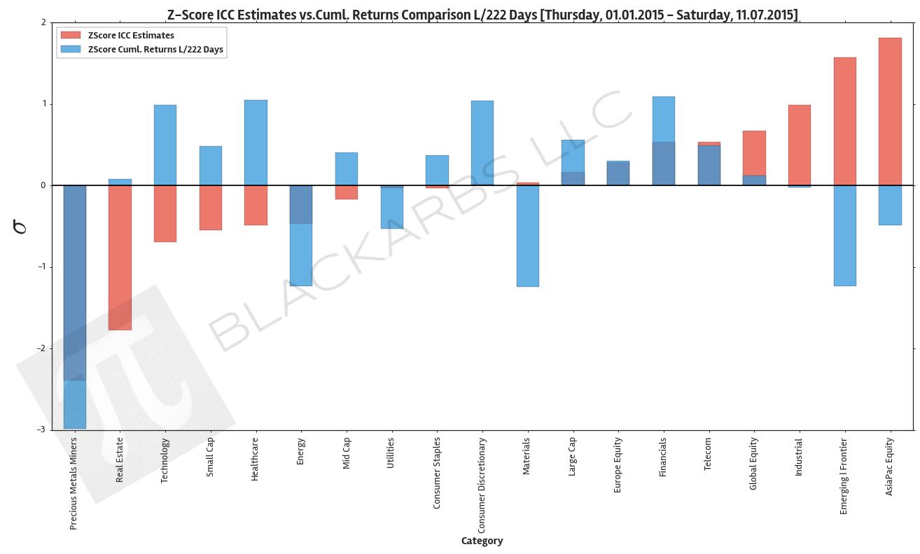
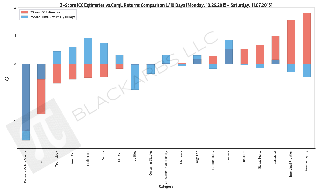
The below plot gives visual representation of the ICC estimates. I z-scored both year-to-date cumulative returns and the ICC estimates so we can view them on the same scale. Examining this chart allows investors to quickly determine which market sectors are outperforming (underperforming) their respective Implied Cost of Capital Estimates.
The extreme cases show where there are disconnects between the analyst community's forward earnings expectations and actual market performance. The plot is sorted left to right by ascending ICC estimates.
Data Sources: YCharts.com, Yahoo Finance
Data Sources: YCharts.com, Yahoo Finance
Data Sources: YCharts.com, Yahoo Finance
Data Sources: YCharts.com, Yahoo Finance
Data Sources: YCharts.com, Yahoo Finance
Long term growth rate (g) is assumed to be 2.5% reflective of our low growth high debt economic environment.
Earlier this year I used to publish a bi-weekly article using the "Implied Cost of Capital" model as an ETF relative value estimation tool. Unfortunately State Street began reporting obvious erroneous data points and eventually stopped providing certain fundamental data altogether. As a result I had to suspend publishing of my ICC estimates.
Well thanks to YCharts.com and their excellent site I was able to find the requisite data needed to begin publishing my model estimates again.
“In accounting and finance the implied cost of equity capital (ICC)—defined as the internal rate of return that equates the current stock price to discounted expected future dividends—is an increasingly popular class of proxies for the expected rate of equity returns. ”
To see a more involved explanation of the previous model I used see here.
In the past I used a Multi-Stage Residual Income Model. However, this time around I've decided to use a simpler Single-Stage Residual Income Model for these estimates. I chose this because I believe the additional complexity is not warranted given my purpose which I will elaborate on further.
The Single-Stage Residual Income Model as defined by the CFA Institute is the following:
source: CFA Institute
'V' is the stock price at time 0, 'B' is the book value of equity at time 0, 'ROE' is return on equity, 'g' is an assumed long term growth rate and 'r' is the cost of equity/capital. The ICC model essentially solves for 'r' given the other inputs.
There is ongoing debate regarding the ICC model's application and accuracy as a proxy for expected returns as quoted by Charles C. Y. Wang. As an investor/trader I'm less interested in the academic debate and more intrigued by the intuition behind the model and its practical application as a relative value tool.
For this purpose I believe it provides great insight.
Long term growth rate (g) is assumed to be 2.5% reflective of our low growth high debt economic environment.
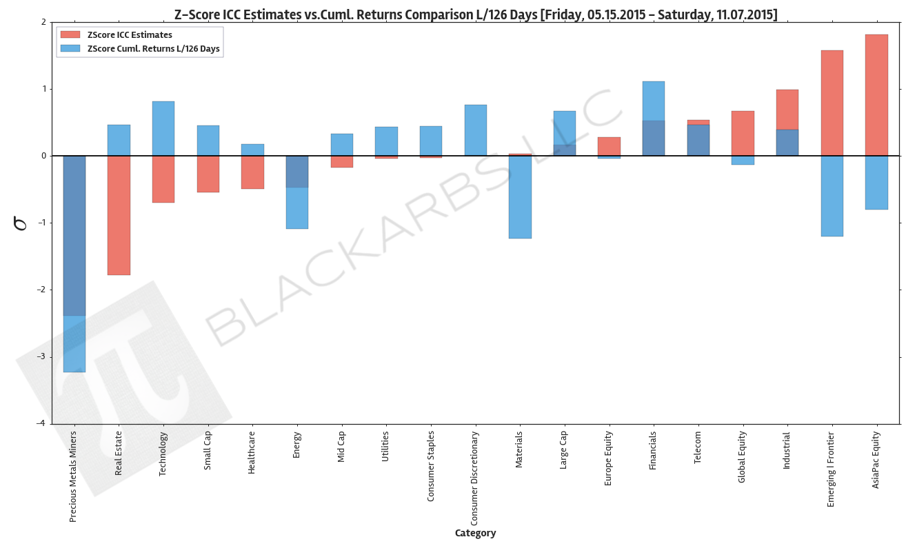
The below plot gives visual representation of the ICC estimates. I z-scored both year-to-date cumulative returns and the ICC estimates so we can view them on the same scale. Examining this chart allows investors to quickly determine which market sectors are outperforming (underperforming) their respective Implied Cost of Capital Estimates.
The extreme cases show where there are disconnects between the analyst community's forward earnings expectations and actual market performance. The plot is sorted left to right by ascending ICC estimates.

Data Sources: YCharts.com, Yahoo Finance
To this day the most popular article I have ever written on this blog was "How to get Free Intraday Stock Data with Netfonds". Unfortunately the Netfonds API has really declined in terms of usability, with too many popular stocks missing, and irregular trade and price quotes. Simply put, as the API went down, so did the code.
However, all hope is not lost. The wonderful people at BarChart.com have created a well documented, easily accessible API for intraday stock data and even near real-time quote access. The only caveat is that you must request access to get a personal API key. Again this is FREE, and the process is extremely simple and straightforward. I think I received my API key within the same day, max 24 hours.
Step 1: Go to http://www.barchartondemand.com/api.php and request an API key.
Step 2: Use or modify my code to get FREE intraday stock data.
Something to note, in this example I use the SP500 components as my list of stock symbols. I covered how to get fresh SPY holdings data directly from the provider in a previous post titled "GET FREE FINANCIAL DATA W/ PYTHON (STATE STREET ETF HOLDINGS - SPY)". Now onto the code...
First I import the necessary modules.
# -*- coding: utf-8 -*-
import time
t0 = time.clock()

import pandas as pd
from pandas.tseries.offsets import BDay
import numpy as np
import datetime as dt
from copy import copy
import warnings
warnings.filterwarnings('ignore',category=pd.io.pytables.PerformanceWarning)
Next I set up what I refer to as a 'datetime management' section of my code. I do this for ALL my time series analysis as a convenient way to standardize my code across projects. Sometimes I only use one of the variables, as I do in this case, but it's so convenient when doing any sort of exploratory analysis with time series. I also do the same for my filepaths.
# ================================================================== #
# datetime management

d = dt.date.today()
# ---------- Days ----------
l10 = d - 10 * BDay()
l21 = d - 21 * BDay()
l63 = d - 63 * BDay()
l252 = d - 252 * BDay()
# ---------- Years ----------
l252_x2 = d - 252 * 2 * BDay()
l252_x3 = d - 252 * 3 * BDay()
l252_x5 = d - 252 * 5 * BDay()
l252_x7 = d - 252 * 7 * BDay()
l252_x10 = d - 252 * 10 * BDay()
l252_x20 = d - 252 * 20 * BDay()
l252_x25 = d - 252 * 25 * BDay()

# ================================================================== #
# filepath management

project_dir = r'D:\\'
price_path = project_dir + r'Stock_Price_Data\\'
Next I set up a convenience function for creating the BarChart url to access the API.
# ================================================================== #
apikey = 'insert_your_api_key'
def construct_barChart_url(sym, start_date, freq, api_key=apikey):
    '''Function to construct barchart api url'''

    url = 'http://marketdata.websol.barchart.com/getHistory.csv?' +\
            'key={}&symbol={}&type={}&startDate={}'.format(api_key, sym, freq, start_date)
    return url
Now for the fun part. I create a function that does the following:
def get_minute_data():
    '''Function to Retrieve <= 3 months of minute data for SP500 components'''

    # This is the required format for datetimes to access the API
    # You could make a function to translate datetime to this format
    start = '20150831000000'
    #end = d
    freq = 'minutes'
    prices = {}
    symbol_count = len(syms)
    N = copy(symbol_count)
    try:
        for i, sym in enumerate(syms, start=1):
            api_url = construct_barChart_url(sym, start, freq, api_key=apikey)
            try:
                csvfile = pd.read_csv(api_url, parse_dates=['timestamp'])
                csvfile.set_index('timestamp', inplace=True)
                prices[sym] = csvfile
            except:
                continue
            N -= 1
            pct_total_left = (N/symbol_count)
            print('{}..[done] | {} of {} symbols collected | percent remaining: {:>.2%}'.format(\
                                                                sym, i, symbol_count, pct_total_left))
    except Exception as e:
        print(e)
    finally:
        pass
    px = pd.Panel.from_dict(prices)

    return px
Now I import our list of stock symbols, make some minor formatting edits and run the code.
# ================================================================== #

# header=3 to skip unnecesary file metadata included by State Street
spy_components = pd.read_excel(project_dir +\
                             '_SPDR_holdings/holdings-spy.xls', header=3)
syms = spy_components.Identifier.dropna()
syms = syms.drop(syms.index[-1]).order()

pxx = get_minute_data()
This script takes roughly 40 minutes to run, longer if you try to get the full 3 months they provide, less if you need less data.
Now let's test our output to make sure we got what we expected.
print(pxx)
print(pxx['AAL'].tail())
print(pxx['ZTS'].tail())
The code ran correctly it appears, and the output is what we expected. One thing you may have noticed is that time stamps are not 'EST'. If you want to convert them use the following one liner.
# convert timestamps to EST
pxx.major_axis = pxx.major_axis.tz_localize('utc').tz_convert('US/Eastern')
There is one last consideration that is easy to overlook if you're unfamiliar with some of the technical challenges of 'big data'. When you first run a script like this it is tempting to use the usual storage techniques that pandas provides such as 'pd.to_csv()' or 'pd.to_excel()'. However, consider the volume of data we just collected: 502 (items) x 5866 (major_axis) x 7 (minor_axis) = 20,613,124.
Look at it again and consider this simple code collected over 20 million data points! I ran into trouble with Python/Excel I/O with only 3.5 million data points in the past. Meaning importing and exporting the data took minutes. That's a serious hangup for any type of exploratory research, especially if you plan on sharing and/or collaborating using this dataset.
Pandas HDF5 file storage format to the rescue! Feel free to investigate the power, speed and scalability of HDF5 via the Pandas docs or any of the numerous quality blogs out there accessible by a google search. Needless to say, I/O was reduced from several minutes both ways to seconds. Here is the code I used to store the panel.
try:
    store = pd.HDFStore(price_path + 'Minute_Symbol_Data.h5')
    store['minute_prices'] = pxx
    store.close()
except Exception as e:
    print(e)
finally:
    pass
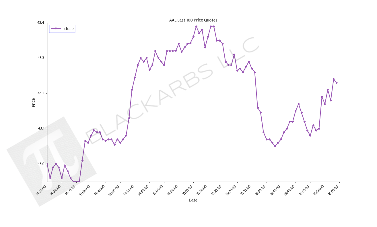
Here's a sample plot with the intraday data.
The entire code is posted below using Gist.

AFFILIATE LINK
Powered by Squarespace