Bernanke's Bluff, Congress Gridlock, What Happens Next?

ben-bernanke_0.jpg

Did you fall for it? Market pundits and the general investment community gave the impression that Bernanke would announce the taper plan during September's FOMC meeting. While not an impossible event, the political and economic situation made it a low probability event. Here are my thoughts on why:

  1. Bernanke's term ends January 31, 2014. A replacement has not been named and at the time one of the key front runners, Larry Summers, withdrew from the race. A policy change to the QE program which has been in place almost continuously since 2009 requires a stable Federal Reserve front office. At minimum market participants needed a clear replacement whose platform they can understand and factor into their investment thesis.
  2. As we can see now, the federal government has fallen into partisan bullshit. Whichever "side" you're on is irrelevant but as a market participant the government shutdown has created uncertainty. At the time Bernanke and the Fed clearly saw the possibility of a government shutdown as a likely destabilizing force in the marketplace.  Uncertainty creates volatility and Bernanke has sought to avoid increasing volatility at all costs.

Not too complicated is it? The Federal Reserve hates volatility. These two forces are the most likely to add to the increase in volatility once the taper is announced. Therefore it is my opinion that any taper announcements with dates and clear reduction amounts will not be declared until the two aformentioned situations are resolved.

In short I expect no taper until a new chairman is named, and the partisan nonsense is resolved/delayed for another year.

As for what happens next, until the government shutdown has concluded expect more volatility. I am still investing/trading with a long bias. As long as the flow of funds from the Federal Reserve continues at the current pace, and economic data continues to show improvement declines in the broad market present opportunities to buy your favorite stock at a discount.

3d Printer Wars - An Industry Primer

3d-Printer-Wars.jpg

Here is a presentation I created focusing on the Additive Manufacturing Industry aka the 3d Printing Industry. I will examine individual firms within the 3d printing industry in an ongoing effort to look for potential profit opportunities in this revolutionary space.

Is Trading the FED's POMO Schedule Profitable?

I often consider the market's distortions that are or can be created by its participants. Arguably, the most important market player is the Federal Reserve. For years the FED as been injecting liquidity into the financial system through its Permanent Open Market Operations (POMO). I'm not going to delve into the purpose of these multibillion dollar transactions as others have covered this extensively. Instead I ask a simple question. The FED makes their tentative POMO schedule public beforehand. Can a trader simply buy the market open and sell the close each day the FED engages in POMO and earn a profit? The simple answer is 'yes'! To set up this study; I compared the FED"s historical POMO calender  from January 2010 until August 3rd 2013 , to S&P 500 (SPX) returns for the matching dates. The return is based on a trader purchasing the SPX on open and closing the position at the end of day. I've provided the histogram of returns below along with an overlay of the density plot.

Histogram Transaction Day

We can see that the returns have a slight negative skew with a couple >-4% days. Additionally the mode is just to the right of zero between 0 and 1%..  For context, the simple annualized sharp ratio is 0.51. Not great but slightly positive. I wondered if there could be a simple improvement to the strategy. What if the SPX trade was instead executed on the POMO settlement day which occurs the next trading day?  The histogram below plots the return results.

Settlement Histogram

To my surprise this strategy was a large improvement. First there were no days with negative returns in excess of -4%. The mode is clearly positive approximating 2.5% and there appears to be a slight positive skew. For comparison the annualized Sharpe ratio is 1.76-Definitely respectable. Looking at the performance summary helps to compare the strategies. The first panel is a wealth index based on the cumulative value of $1 over the period. Clearly the settlement date strategy blows away the transaction date strategy by 40+% with a drawdown not exceeding 10% over the testing period.

POMO perf summary


Let me emphasize that the strategy may or may not be tradable today. On a superficial basis the strategy appears to be promising, But further research and more indepth analysis would have to be done, analyzing actual transactions, portfolio size, scale, and so on.

To construct the charts and run my analysis I used R!'s GGPLOT2 and PerformanceAnalytics packages along with Moments, Scales, and Quantmod.

Using R to Chart Shadow Banking Components

Previously I wrote a primer on the shadow banking markets. In this post I follow up by attempting to chart and analyze the components. Surprisingly (or not) it proved more difficult than I anticipated to construct the components charts. First finding good data series that could serve as a proxy was time consuming. Additionally some of the data series that helped in deconstructing the market in the past were discontinued. I also had to merge data from several sources. Keep in mind this is definitely far from exact but does provide a good guideline. Without further ado here are the charts generated using Rstudio and ggplot2 packages. SBC stacked bar


This is the components chart constructed using quarterly data. As you can see the chart is uneven for the most recent data as some of the time series have not been updated as quickly as others. The first aspect to note is the multi trillion dollar drop off beginning in early 2010 comprised almost entirely of Agency and GSE mortgage pools disappearing from the market. No wonder the Federal Reserve had to step in and purchase these assets to clear the Bank's and Non-Bank's books. That much asset liquidation would have bankrupted a lot of global financial entities. 

 **I was unable to reconcile my aggregated components data with the Financial Stability Boards' $24 trillion dollar market size estimate. If anyone has any ideas to contribute for increasing the accuracy of this chart, or data series they feel should be included let me know.**


SBC Grid Plot


Here is the previous chart deconstructed to illustrate the size of the shdadow banking compenents individually. This further showcases the total collapse in the Agency/GSE mortgage pool arena. Again it would appear the primary dealers are the largest and most consistent players in this marketfollowed by Money Market Funds and ABS Issuers. 


gcf repo rates


Just for fun I have included the DTCC's GCF Repo Index Rates. You can see the steady climb from 2005 to 2007 and then the drop off beginning in late '07. I haven't done enough research to explain the dramatic collapse in rates definitively. However, my guess is that the implicit (explicit) guarantee of the underlying collateral by the Federal Reserve, via a myriad of alphabet credit facilities it extended to global financial instituations during that time period, led to the stabilization of repo rates.


Some Notes:

To construct the component charts I queried the open source Quandl database which contained data from the FRED database. Here are the R queries:

mf = Quandl('FRED/MMMFTCMAHDFS', collapse='quarterly', start_date='2002-01-01') repo = Quandl('FRED/OLRACBM027NBOG', collapse='quarterly', start_date='2002-01-01') abs = Quandl('FRED/ABSITCMDODFS', collapse='quarterly', start_date='2002-01-01') agse = Quandl('FRED/AGSEMPTCMDODFS', collapse='quarterly', start_date='2002-01-01') fc = Quandl('FRED/FUCTCMDODFS',collapse='quarterly', start_date='2002-01-01') cp = Quandl('FRED/COMPUTN',collapse='quarterly', start_date='2002-01-01')

To gather the Primary Dealer data I used the Federal Reserve of New York's website; which I then had to manipulate to match the datapoints of the closest available date to the FRED data.

The packages I used to construct the charts in Rstudio are the following:

library(ggplot2) library(reshape2) library(Quandl) library(scales) library(reshape)

If anyone is interested in the code let me know and I'll paste it to this post.

Shadow Banking _ A primer

shadow-banking.jpg

How large is this shadow banking market??

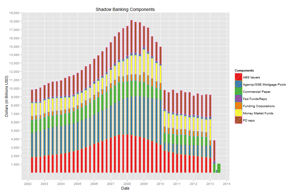
Estimates vary due to the inherent difficulty of quantifying ‘shadow’ assets. The most recent figures cited by the Federal Reserve and computed by the financial stability board has pegged the global shadow market at approximately $65 trillion USD; having peaked in 2007 at 128% of aggregate GDP* now settling in at approximately 111%.

Of the $65 trillion shadow market, the U.S. accounts for an estimated 35% or ~$23 trillion followed by the euro area at $22 trillion and UK at $9 trillion.

*aggregate GDP of 20 jurisdictions and the Euro area at end-2011

What is shadow banking?

Shadow banking is the unregulated creation of credit by regulated and unregulated entities. The ‘shadow’ moniker makes reference to the fact that this credit creation is often facilitated off-balance sheet and often difficult to quantify. The criteria for shadow banking activities is as follows:

  1. Credit intermediation - facilitating transactions between lenders and borrowers

  2. Maturity/liquidity transformation - fund long-term assets with short-term liabilities/illiquid assets funded by liquid liabilities

  3. Lack of government guarnatee/access to central bank liquidity

  4. Outside the regulated banking system

  5. Credit risk transfer

Who participates in the shadow banking market?

The primary facilitators and lenders in this market include: hedge funds, bank holding companies, global asset managers, money market mutual funds; their subsidiaries via special purpose entities (SPE’s), structured investment vehicles (SIV’s), and other non-bank financial institutions including pension funds, endowments, insurance firms et al. On the other side are the borrowers who range from corporations to the aforementioned non-bank financial institutions.

How do shadow banks and traditional banks differ?

Traditional banks fund their loans via deposits whereas shadow banks use short term funding commonly provided by asset backed commercial paper and repo markets. There are other strategies to facilitate this funding but they are beyond the scope of this post.  The lack of deposit taking is what allows these entities to evade traditional regulatory burden. This often translates to lower rates for the borrower when compared to  traditional loan mechanisms. Lower fees = popularity = increasing market share/size.

I’m confused, what are asset backed commercial paper and repo agreements?

Asset backed commercial paper functions like a pass through debt security with maturities typically between 1 and 270 days. Companies looking to increase liquidity sell a portfolio of receivables to “banks” who then securitize the cash flows and sell them to investors. As the cash flows for the receivables are paid to the company they pass them along the chain, via the “bank” who in turn redistributes the funds to the investors.

EXAMPLE:

Bell computers sells receivables to ⇒⇒ Oldman Scratch bank who packages and sells to  ⇒⇒  Investors

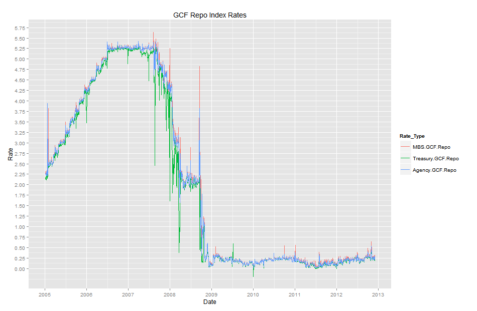
Repurchase agreements also function as short term funding vehicles. It works when a  firm  sells collateral  (usually some other debt or equity security) to a buyer.  Accompanying this  sale and purchase is a contractual agreement where the seller agrees to buy the collateral back at a later date and a higher price. The difference in price is effectively the interest rate on the cash flows. This is commonly called the repo rate.

EXAMPLE:

Phase 1_

Company A needs cash and sells collateral to ⇒⇒firm B who buys or effectively loans company A the money while taking legal ownership of the collateral

Phase 2_

@ maturity company A buys back the collateral at the agreed upon price effectively returning the principal plus interest ⇒⇒ firm B collects the cash  and returns the collateral and legal ownership.

Why is this important??

This is important because there are ~$65 trillion in assets that operate outside of traditional regulation. The shadow banking market was shown to play a pivotal role in the financial meltdown as the generationally low interest rates at the time did NOT compensate investors and/or lenders for increasing risk. As a result many of these sub sectors within the shadow market grinded to a halt as lenders refused to roll over debt. Rates blew out, and firms had to liquidate assets at ‘fire sale’ prices in order to pay their liabilities. Adding to the problem was the interconnectedness of these firms. The shadow market contained assets and liabilities that were seemingly impossible to quantify and assign. This created a negative feedback loop in the market as people did not know who owed who, whose assets were money good or completely illiquid, or worse-completely worthless.

The shadow banking market is not growing at the pace it once was but it is incredibly influential. A sophisticated investor must be aware that it exists and is large and find ways to keep track. Dislocations in the shadow market often provide profitable opportunities. In future posts I will breakdown some useful proxies to help track this market.